|
|
|
|
As pointed in About,
" urge the reader to use/trust the content only after verifying it against standards and/or consulting it with experts in the field".
|
»
|
|
MATLAB resources
|
|
Best resources to learn and use MATLAB are available on their website
(documentation, examples, tutorials, queries-n-answers).
To begin with, you may start with below tutorial page
|
MATLAB tutorials
|
|
There is also "Get Started" page.
|
MATLAB Get Started
|
|
|
»
|
|
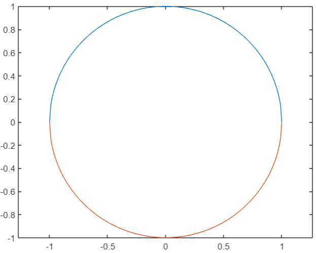
Draw a Circle in MATLAB
|
x = -1:1/100:1;
plot(x, sqrt(1 - x .* x))
hold on
plot(x, -sqrt(1 - x .* x))
axis equal
hold off
|
|
|
|
»
|
|
Draw a Cylinder in MATLAB
|
R = 2;
N = 10;
x = -R:R/N:R;
y = sqrt(R*R - x .* x);
z = ones(N*2+1,1) * x;
z = z';
surf(x,y,z)
axis equal
hold on
Y = -sqrt(R*R - x .* x);
surf(x,Y,z)
hold off

|
|
|
|
»
|
|
Draw a Sphere in MATLAB
|
N = 50;
R = 2;
theta = 0:pi/N:pi;
phi = 0:pi/N:pi;
[th, ph] = meshgrid(theta,phi);
X = sin(th).*cos(ph);
Y = sin(th).*sin(ph);
Z = cos(th);
surf(R*X,R*Y,R*Z);
axis equal
hold on
surf(R*X,-R*Y,R*Z);
hold off

|
|
|
|
»
|
|
Quadratic polynomial
|
%% Quadratic polynomial f(x) = x^2 - 8x + 20
%% with roots: 4 + j2 and 4 - j2
x = 0:.25:6;
y = -3:.25:3;
[X, Y] = meshgrid(x,y);
A = zeros(size(X));
for c1 = 1:size(X,1)
for c2 = 1:size(X,2)
Number = X(c1,c2) + 1i * Y(c1, c2);
A(c1, c2) = abs(Number^2 - 8*Number + 20);
end
end
f_of_x = mesh(X, Y, A);
xlabel('real');
ylabel('imag');
zlabel('f(x)');

|
|
|
|
»
|
|
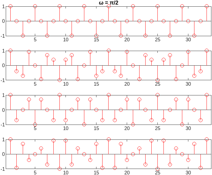
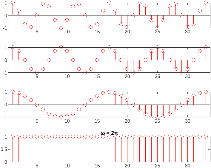
Discrete-Time Sinusoid
|
%% Disrete Sinusoid frequency
n = -16:1:16;
F1 = figure('Visible','off');
color = 'red';
marker = 'o';
tiledlayout(4,1);
nexttile;
w = 0;
S = stem(cos(w*n));
S.Color = color;
S.Marker = marker;
title('ω = 0');
nexttile;
w = w + pi/8;
S = stem(cos(w*n));
S.Color = color;
S.Marker = marker;
nexttile;
w = w + pi/8;
S = stem(cos(w*n));
S.Color = color;
S.Marker = marker;
nexttile;
w = w + pi/8;
S = stem(cos(w*n));
S.Color = color;
S.Marker = marker;
exportgraphics(F1, 'dsp_discrete_sinusoid_1.png');
F2 = figure('Visible','off');
tiledlayout(4,1);
nexttile;
w = w + pi/8;
S = stem(cos(w*n));
S.Color = color;
S.Marker = marker;
title('ω = π/2');
nexttile;
w = w + pi/8;
S = stem(cos(w*n));
S.Color = color;
S.Marker = marker;
nexttile;
w = w + pi/8;
S = stem(cos(w*n));
S.Color = color;
S.Marker = marker;
nexttile;
w = w + pi/8;
S = stem(cos(w*n));
S.Color = color;
S.Marker = marker;
exportgraphics(F2, 'dsp_discrete_sinusoid_2.png');
F3 = figure('Visible','off');
tiledlayout(4,1);
nexttile;
w = w + pi/8;
S = stem(cos(w*n));
S.Color = color;
S.Marker = marker;
title('ω = π');
exportgraphics(F3, 'dsp_discrete_sinusoid_3.png');
F4 = figure('Visible','off');
tiledlayout(4,1);
nexttile;
w = w + pi/8;
S = stem(cos(w*n));
S.Color = color;
S.Marker = marker;
nexttile;
w = w + pi/8;
S = stem(cos(w*n));
S.Color = color;
S.Marker = marker;
nexttile;
w = w + pi/8;
S = stem(cos(w*n));
S.Color = color;
S.Marker = marker;
nexttile;
w = w + pi/8;
S = stem(cos(w*n));
S.Color = color;
S.Marker = marker;
title('ω = 3π/2');
exportgraphics(F4, 'dsp_discrete_sinusoid_4.png');
F5 = figure('Visible','off');
tiledlayout(4,1);
nexttile;
w = w + pi/8;
S = stem(cos(w*n));
S.Color = color;
S.Marker = marker;
nexttile;
w = w + pi/8;
S = stem(cos(w*n));
S.Color = color;
S.Marker = marker;
nexttile;
w = w + pi/8;
S = stem(cos(w*n));
S.Color = color;
S.Marker = marker;
nexttile;
w = w + pi/8;
S = stem(cos(w*n));
S.Color = color;
S.Marker = marker;
title('ω = 2π');
exportgraphics(F5, 'dsp_discrete_sinusoid_5.png');


|
|
|
|
»
|
|
Sampling of a sinusoid
|
%% sampling
granularity = 2^12;
time = 0:pi/granularity:1;
sampling_frequency = 32;
number_of_sampling_values = size(time, 2)/sampling_frequency;
F = figure('Visible','off');
color = 'red';
marker = 'o';
tiledlayout(4,1);
nexttile;
frequency = 1;
P = plot(cos(2*pi*time*frequency));
P.Color = color;
title("frequency = " + frequency);
xticklabels([]);
nexttile;
cosine_values = cos(2*pi*time*frequency);
sampled = cosine_values(1:number_of_sampling_values:end);
S = stem(sampled);
S.Color = color;
S.Marker = marker;
title("sampling frequency = " + sampling_frequency);
nexttile;
frequency2 = 2;
P = plot(cos(2*pi*time*frequency2));
P.Color = color;
title("frequency = " + frequency2);
xticklabels([]);
nexttile;
cosine_values = cos(2*pi*time*frequency2);
sampled = cosine_values(1:number_of_sampling_values:end);
S = stem(sampled);
S.Color = color;
S.Marker = marker;
title("sampling frequency = " + sampling_frequency);
exportgraphics(F, 'dsp_sampling.png');

|
|
|
|
»
|
|
Aliasing
|
%% aliasing
granularity = 2^12;
time = 0:pi/granularity:1;
sampling_frequency = 32;
number_of_sampling_values = size(time, 2)/sampling_frequency;
F = figure('Visible','off');
color = 'red';
marker = 'o';
tiledlayout(4,1);
nexttile;
frequency = 2;
p = plot(cos(2*pi*time*frequency));
p.Color = color;
title("frequency = " + frequency);
xticklabels([]);
nexttile;
cosine_values = cos(2*pi*time*frequency);
sampled = cosine_values(1:number_of_sampling_values:end);
S = stem(sampled);
S.Color = color;
S.Marker = marker;
title("sampling frequency = " + sampling_frequency);
nexttile;
frequency2 = (sampling_frequency/2) + (sampling_frequency/2 - frequency);
P = plot(cos(2*pi*time*frequency2));
P.Color = color;
title("frequency = " + frequency2);
nexttile;
cosine_values = cos(2*pi*time*frequency2);
sampled = cosine_values(1:number_of_sampling_values:end);
S = stem(sampled);
S.Color = color;
S.Marker = marker;
title("sampling frequency = " + sampling_frequency);
exportgraphics(F, 'dt_aliasing.png');

|
|
|
|
»
|
|
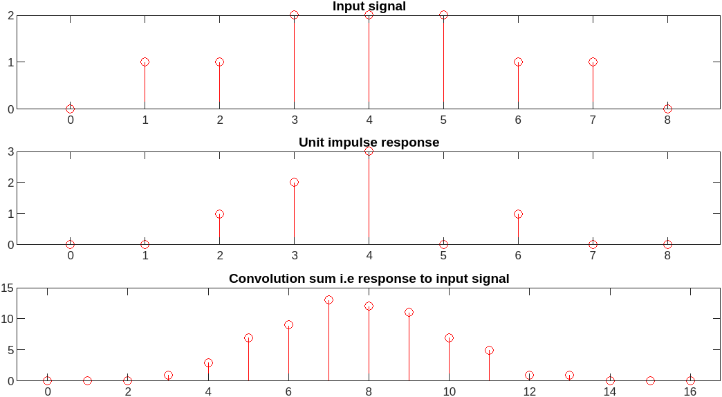
Discrete-Time Convolution sum
|
%% Discrete-time Convolution sum
sample_n1 = 0:1:8;
unit_impulse_reponse = [ 0 0 1 2 3 0 1 0 0];
input_signal = [ 0 1 1 2 2 2 1 1 0 ];
convolution_sum = conv (input_signal, unit_impulse_reponse);
sample_n2 = 0:length(convolution_sum)-1;
F = figure('Visible','off');
F.Position(3) = F.Position(3) * 1.5;
number_of_plots = 3;
plot_ctr = 0;
color = 'red';
marker = 'o';
plot_ctr = plot_ctr + 1;
subplot(number_of_plots,1,plot_ctr)
S = stem(sample_n1, input_signal);
S.Color = color;
S.Marker = marker;
title('Input signal')
plot_ctr = plot_ctr + 1;
subplot(number_of_plots,1,plot_ctr)
S = stem(sample_n1, unit_impulse_reponse);
S.Color = color;
S.Marker = marker;
title('Unit impulse response');
plot_ctr = plot_ctr + 1;
subplot(number_of_plots,1,plot_ctr)
S = stem(sample_n2, convolution_sum);
S.Color = color;
S.Marker = marker;
title('Convolution sum i.e response to input signal');
exportgraphics(F, 'dt_convolution_example.png');
|
|
|
|
»
|
|
Discrete-Time Signal Operations
|
%% Discrete-time Signal operations
%% odd number of elements so we get zero in the middle
y_n = [ 0 0 0 1 2 3 4 0 0 0 0 0 0 ];
y_minus_n = zeros(size(y_n));
for c1 = 1:size(y_n, 2)
n = c1 - fix(size(y_n, 2)/2) - 1;
new_n = -n;
new_c1 = new_n + 1 + fix(size(y_n, 2)/2);
y_minus_n(1, c1) = y_n(1, new_c1);
end
y_n_plus_k = zeros(size(y_n));
plus_k = 2;
for c1 = 1:size(y_n, 2) - plus_k
n = c1 - fix(size(y_n, 2)/2) - 1;
new_n = n + plus_k;
new_c1 = new_n + 1 + fix(size(y_n, 2)/2);
y_n_plus_k(1, c1) = y_n(1, new_c1);
end
y_n_minus_k = zeros(size(y_n));
minus_k = 2;
for c1 = (minus_k+1):size(y_n, 2)
n = c1 - fix(size(y_n, 2)/2) - 1;
new_n = n - minus_k;
new_c1 = new_n + 1 + fix(size(y_n, 2)/2);
y_n_minus_k(1, c1) = y_n(1, new_c1);
end
y_minus_n_plus_k = zeros(size(y_n));
plus_k = 2;
for c1 = (plus_k+1):size(y_n, 2)
n = c1 - fix(size(y_n, 2)/2) - 1;
new_n = - n + plus_k;
new_c1 = new_n + 1 + fix(size(y_n, 2)/2);
y_minus_n_plus_k(1, c1) = y_n(1, new_c1);
end
y_n_down_sampling_by_k = zeros(size(y_n));
down_sampling_by_k = 2;
for c1 = 1:size(y_n, 2)
n = c1 - fix(size(y_n, 2)/2) - 1;
new_n = n * down_sampling_by_k;
new_c1 = new_n + 1 + fix(size(y_n, 2)/2);
if (new_c1 >=1) && (new_c1 <= size(y_n, 2))
y_n_down_sampling_by_k(1, c1) = y_n(1, new_c1);
end
end
y_n_scale_by_A = zeros(size(y_n));
scale_by_A = 2;
for c1 = 1:size(y_n, 2)
y_n_scale_by_A(1, c1) = scale_by_A * y_n(1, c1);
end
%% "fix" will get you integer portion of fraction
sample_n1 = (0 - fix(size(y_n, 2)/2)):1:(fix(size(y_n, 2)/2));
color = 'red';
marker = 'o';
F1 = figure('Visible','off');
tiledlayout(4,1);
nexttile;
S = stem(sample_n1, y_n);
S.Color = color;
S.Marker = marker;
title('h(n)')
nexttile;
S = stem(sample_n1, y_minus_n);
S.Color = color;
S.Marker = marker;
title('Folding: h(-n)')
nexttile;
S = stem(sample_n1, y_n_plus_k);
S.Color = color;
S.Marker = marker;
title("Shifting Advance: h(n+k), k=" + plus_k)
nexttile;
S = stem(sample_n1, y_n_minus_k);
S.Color = color;
S.Marker = marker;
title("Shifting Delay: h(n-k), k=" + minus_k)
exportgraphics(F1, 'dt_signal_operations_1.png');
F2 = figure('Visible','off');
tiledlayout(4,1);
nexttile;
S = stem(sample_n1, y_minus_n_plus_k);
S.Color = color;
S.Marker = marker;
title("Folding & Shifting: h(-n+k), k=" + plus_k)
nexttile;
S = stem(sample_n1, y_n_down_sampling_by_k);
S.Color = color;
S.Marker = marker;
title("Down-sampling or Time scaling: h(n*k), k=" + down_sampling_by_k)
nexttile;
S = stem(sample_n1, y_n_scale_by_A);
S.Color = color;
S.Marker = marker;
title("Amplitude scaling: A * h(n), A=" + scale_by_A)
exportgraphics(F2, 'dt_signal_operations_2.png');


|
|
|
|
»
|
|
Discrete-Time Crosscorrelation
|
%% Discrte-Time Crosscorrelation example
f1_n = [ 0 0 0 0 0 0 4 3 2 1 0 0 0 ];
f2_n = [ 0 0 0 0 0 0 4 4 4 4 0 0 0 ];
f2_minus_n = zeros(size(f2_n));
for c1 = 1:size(f2_n, 2)
n = c1 - fix(size(f2_n, 2)/2) - 1;
new_n = -n;
new_c1 = new_n + 1 + fix(size(f2_n, 2)/2);
f2_minus_n(1, c1) = f2_n(1, new_c1);
end
crosscorrelation_n = conv (f1_n, f2_minus_n);
sample_n1 = (0 - fix(size(f1_n, 2)/2)):1:(fix(size(f1_n, 2)/2));
sample_n2 = (0 - fix(size(crosscorrelation_n, 2)/2)):1:(fix(size(crosscorrelation_n, 2)/2));
color = 'red';
marker = 'o';
F = figure('Visible','off');
tiledlayout(4,1);
nexttile;
S = stem(sample_n1, f1_n);
S.Color = color;
S.Marker = marker;
title('y1(n)')
nexttile;
S = stem(sample_n1, f2_n);
S.Color = color;
S.Marker = marker;
title('y2(n)')
nexttile;
S = stem(sample_n2, crosscorrelation_n);
S.Color = color;
S.Marker = marker;
title('Crosscorrelation: y1(n) * y2(-n)')
exportgraphics(F, 'dt_crosscorrelation_example.png');

|
|
|
|
»
|
|
Discrete-Time Autocorrelation
|
%% Discrte-Time Autocorrelation example
f_n = [ 0 0 0 0 0 0 4 3 2 1 0 0 0];
f_minus_n = zeros(size(f_n));
for c1 = 1:size(f_n, 2)
n = c1 - fix(size(f_n, 2)/2) - 1;
new_n = -n;
new_c1 = new_n + 1 + fix(size(f_n, 2)/2);
f_minus_n(1, c1) = f_n(1, new_c1);
end
autocorrelation_n = conv (f_n, f_minus_n);
sample_n1 = (0 - fix(size(f_n, 2)/2)):1:(fix(size(f_n, 2)/2));
sample_n2 = (0 - fix(size(autocorrelation_n, 2)/2)):1:(fix(size(autocorrelation_n, 2)/2));
color = 'red';
marker = 'o';
F = figure('Visible','off');
tiledlayout(4,1);
nexttile;
S = stem(sample_n1, f_n);
S.Color = color;
S.Marker = marker;
title('y(n)')
nexttile;
S = stem(sample_n1, f_minus_n);
S.Color = color;
S.Marker = marker;
title('Folding: y(-n)')
nexttile;
S = stem(sample_n2, autocorrelation_n);
S.Color = color;
S.Marker = marker;
title('Autocorrelation: y(n) * y(-n)')
exportgraphics(F, 'dt_autocorrelation_example.png');

|
|
|
|
»
|
|
Discrete-Time Autocorrelation to find Periodicity
|
%% Discrte-Time Autocorrelation to find periodicity
f1_n = [ 4 3 2 1 0 4 3 2 1 0 4 3 2 1 0 4 3 2 1 0 4 ];
f2_n = [ 0 0 0 1 1 0 0 0 0 0 1 2 1 1 0 0 0 0 0 0 0 ];
f3_n = zeros(size(f1_n));
for c1 = 1:size(f1_n, 2)
f3_n(1, c1) = f1_n(1, c1) + f2_n(1, c1);
end
f3_minus_n = zeros(size(f3_n));
for c1 = 1:size(f3_n, 2)
n = c1 - fix(size(f3_n, 2)/2) - 1;
new_n = -n;
new_c1 = new_n + 1 + fix(size(f3_n, 2)/2);
f3_minus_n(1, c1) = f3_n(1, new_c1);
end
autocorrelation_f3_n = conv (f3_n, f3_minus_n);
sample_n1 = (0 - fix(size(f1_n, 2)/2)):1:(fix(size(f1_n, 2)/2));
sample_n2 = (0 - fix(size(autocorrelation_f3_n, 2)/2)):1:(fix(size(autocorrelation_f3_n, 2)/2));
color = 'red';
marker = 'o';
F1 = figure('Visible','off');
tiledlayout(4,1);
nexttile;
S = stem(sample_n1, f1_n);
S.Color = color;
S.Marker = marker;
title('f1(n)')
nexttile;
S = stem(sample_n1, f2_n);
S.Color = color;
S.Marker = marker;
title('f2(n)')
nexttile;
S = stem(sample_n1, f3_n);
S.Color = color;
S.Marker = marker;
title('f3(n) = f1(n) + f2(n)')
exportgraphics(F1, 'dt_autocorrelation_to_find_periodicity1.png');
F2 = figure('Visible','off');
tiledlayout(1,1);
nexttile;
S = stem(sample_n2, autocorrelation_f3_n);
S.Color = color;
S.Marker = marker;
title('Autocorrelation: f3(n) * f3(-n)')
exportgraphics(F2, 'dt_autocorrelation_to_find_periodicity2.png');


|
|
|
|
»
|
|
Discrete-Time Exponential signal
|
%% Discrte-Time Exponential signal example
total_samples = 30 + 1;
a_val = 0.9;
last_exp_n = 1;
exp_n = zeros(1,total_samples);
exp_n(1, 1) = last_exp_n;
for n = 2:total_samples
last_exp_n = last_exp_n * a_val;
exp_n(1, n) = last_exp_n;
end
last_negative_exp_n = -1;
negative_exp_n = zeros(1,total_samples-1);
negative_exp_n(1, 1) = last_negative_exp_n;
for n = total_samples-1:-1:1
last_negative_exp_n = last_negative_exp_n * a_val;
negative_exp_n(1, n) = last_negative_exp_n;
end
sample_n = 0:1:(total_samples-1);
sample_minus_n = -(total_samples-1):1:-1;
color = 'red';
marker = 'o';
F = figure('Visible','off');
tiledlayout(2,1);
nexttile;
S = stem(sample_n, exp_n);
S.Color = color;
S.Marker = marker;
title('exp(n), a=0.9')
nexttile;
S = stem(sample_minus_n, negative_exp_n);
S.Color = color;
S.Marker = marker;
title('negative exp(n), a=0.9')
exportgraphics(F, 'dt_crosscorrelation_example.png');

|
|
|
|
»
|
|
Notes
|
|
round
|
Round off to the nearest integer
|
|
floor
|
Apporximate towards −∞ (negative infinity)
|
|
fix
|
Apporximate towards zero
|
|
ceil
|
Round off to the larger integer
|
|
zeror(rows,column)
|
Array with zeros
|
|
|
|
|
»
|
|
Repeated convolutions of Discrete-Time signal with itself
|
%% Repeated convolutions Discrete-Time signal with itself
f1_of_n = [ 0 0 0 0 1 2 5 2 3 2 4 2 1 0 0 0 0 ];
sample_n_f1 = 0:length(f1_of_n)-1;
conv_f1 = conv (f1_of_n, f1_of_n);
conv_f1 = conv (conv_f1, f1_of_n);
conv_f1 = conv (conv_f1, f1_of_n);
sample_n_cv1 = 0:length(conv_f1)-1;
f2_of_n = [ 0 0 0 0 1 2 3 4 5 6 7 8 9 0 0 0 0 ];
sample_n_f2 = 0:length(f2_of_n)-1;
conv_f2 = conv (f2_of_n, f2_of_n);
conv_f2 = conv (conv_f2, f2_of_n);
conv_f2 = conv (conv_f2, f2_of_n);
sample_n_cv2 = 0:length(conv_f2)-1;
F = figure('Visible','off');
F.Position(3) = F.Position(3) * 1.5;
number_of_plots = 4;
plot_ctr = 0;
color = 'red';
marker = 'o';
plot_ctr = plot_ctr + 1;
subplot(number_of_plots,1,plot_ctr)
S = stem(sample_n_f1, f1_of_n);
S.Color = color;
S.Marker = marker;
title('f1(n)');
plot_ctr = plot_ctr + 1;
subplot(number_of_plots,1,plot_ctr)
S = stem(sample_n_cv1, conv_f1);
S.Color = color;
S.Marker = marker;
title('Convolution of f1(n))');
plot_ctr = plot_ctr + 1;
subplot(number_of_plots,1,plot_ctr)
S = stem(sample_n_f2, f2_of_n);
S.Color = color;
S.Marker = marker;
title('f2(n)');
plot_ctr = plot_ctr + 1;
subplot(number_of_plots,1,plot_ctr)
S = stem(sample_n_cv2, conv_f2);
S.Color = color;
S.Marker = marker;
title('Convolution of f2(n))');
exportgraphics(F, 'dt_repeated_convolution.png');

|
|
|
© Copyright Samir Amberkar 2018-24
| |
| |
|
|