|
|
|
|
As pointed in About,
" urge the reader to use/trust the content only after verifying it against standards and/or consulting it with experts in the field".
|
»
|
|
Numbers
|
Below is our number scale. Complex numbers is superset of all numbers.
|

|
|
|
»
|
|
Euler's formula
|

|
|
|
|
»
|
|
IQ Modulation and Demodulation
|
|
In Modulation, Amplitude and Phase of the Carrier is adjusted.
This can be achieved with an "in-phase" component and an "quadrature" component as shown mathematically below.
f is Carrier frequency.
|

|
Demodulation (i.e. getting back "in-phase" and "quadrature" components) is achieved by low pass filter (LPF).
|

|
|
|
»
|
|
Infinite geometric series
|
|
Below series is useful in our analysis.
|

|
|
|
»
|
|
Polynomial
|

|
If a polynomial has real coefficients, its roots are either real or occur in complex conjugate pairs.
|
|
|
»
|
|
Signal processing
|

|

|
Example,
|

|
|
|
»
|
|
Digital Signal Processing system
|

|
|
|
»
|
|
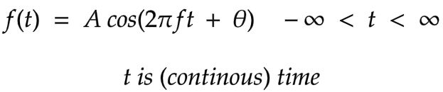
Continuous-Time and Discrete-Time Sinusoid signals
|
|
Continuous-Time
|
|
|
Discrete-Time
|

|
|
|
|
»
|
|
Complex Sinusoid (or Exponential)
|
|
Complex Sinusoid (or Exponential) is a function of frequency and time as shown below.
|

|
If values (complex numbers) are plotted on rectangular coordinates,
it will look like a point revolving in circular motion with frequency f.
Anticlockwise if forward in time, clockwise otherwise.
|

|
|
|
»
|
|
Harmonically related Complex Sinusoids
|
Two sinusoids are said to be harmonically related if their frequencies are multiple of single frequency.
This frequency is known as fundamental frequency.
Below is a linear combination of harmonically related continuous-time sinusoids.
F0 is fundamental frequency.
|

|
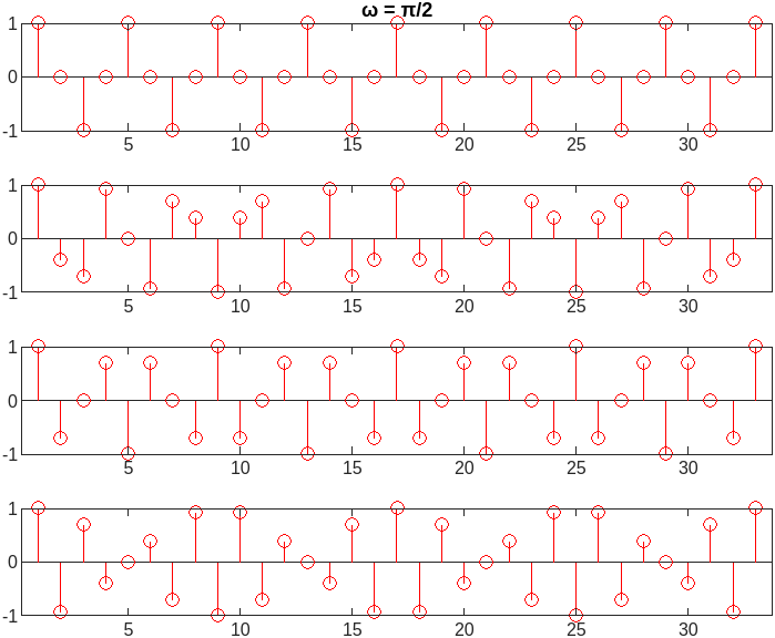
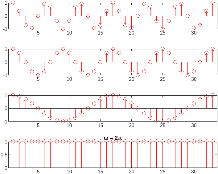
Same combination for discrete-time sinusoids is shown below.
In case of discrete-time sinusoid, as seen earlier, waveforms are same when oscillation rate is separated by 2π.
If N is oscillation period (corresponding to F0), waveforms with k=0 and k=N will be same.
That means, it will be sufficient if we take k from 0 to N-1.
|

|
|
|
|
»
|
|
Sampling of a sinusoid
|
|
Analog to Digital conversion requires Sampling of the analog signal.
Sampling is usually periodic.
Below diagram shows sampling of a sinusoid with two frequencies, but with the same sampling period.
|

|

|
|
|
»
|
|
Sampling theorem
|
|
Below is an equation to get back input analog signal from sampled values.
|

|
|
|
|
»
|
|
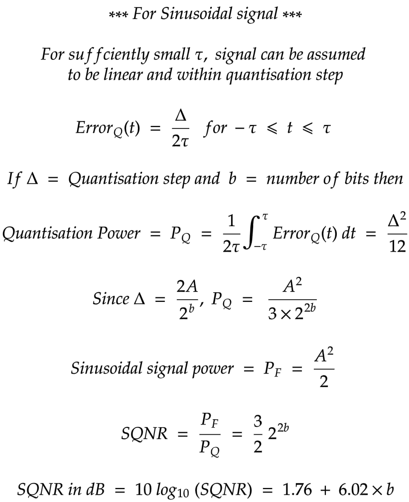
Quantisation
|
During sampling, each sample value of continous-amplitude signal is expressed into certain number of digits (usually bits).
The process is called Quantisation.
Quantisation introduces a certain error due the conversion of continous-value to discrete-value;
this error is known as Quantisation error.
|

|
Information loss due to Quantisation error could be measured in terms of Signal-to-Quantisation noise ratio (SQNR).
Each bit is equivalant to 6 dB power for sinusoidal signal as shown below.
|
|
|
|
|
»
|
|
Elementary discrete-time signals
|
|
Unit impulse
|

|
|
Unit step
|

|
|
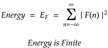
Energy signal
|
|
|
Power signal
|

|
|
Periodic signal
|

|
|
Nonperiodic or Aperiodic signal
|
Signal which is *not* periodic
|
|
Symmetric (even) signal
|

|
|
Antisymmetric (odd) signal
|

|
|
|
|
»
|
|
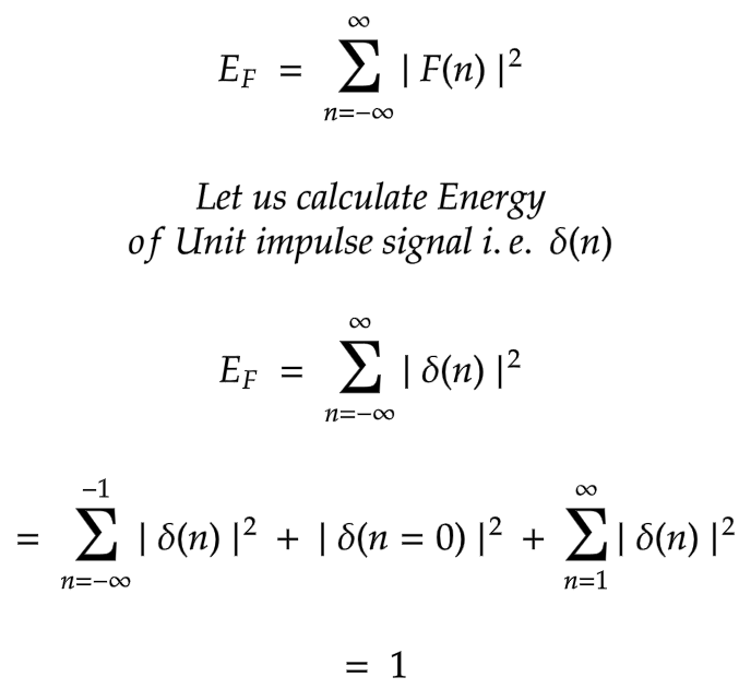
Energy of discrete-time signal
|
|
Below is a definition of Energy and an example calculation for Unit impulse signal.
|
|
As Energy of Unit impulse signal is finite, it is known as an Energy signal.
|
|
|
»
|
|
Power of discrete-time signal
|
|
Below is a definition of Power and an example calculation for Unit step signal.
|

|
As Power of Unit step signal is finite, it is known as Power signal.
|
|
|
»
|
|
Discrete-Time systems
|

|

|
|
|
|
»
|
|
Types of discrete-time systems
|
Static
(memoryless)
|

|
Dynamic
(with memory)
|

|
|
Time invariant
|

|
|
Time variant
|

|
Relaxed or
Not relaxed
|

|
|
Linear
|

|
|
Nonlinear
|
Does *not* satisfy above linear equation.
|
Causal or
Noncausal
|

|
Recursive or
Nonrecursive
|

|
|
Stable
|

|
|
Unstable
|

|
|
|
|
»
|
|
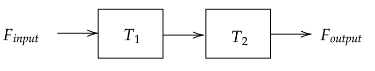
Cascade (Serial) interconnection
|
|

|
|
|
|
»
|
|
Parallel interconnection
|

|

|
|
|
|
»
|
|
Linearity and Time invariance
|
Linearity should be not be related to Time invariance.
Linearity deal with Amplitude or value (y axis) of the signal whereas
Time invariance deal with Time (x axis).
|
|
|
»
|
|
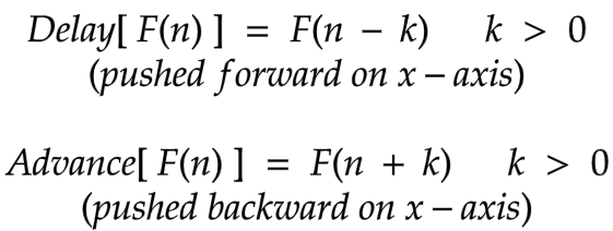
Splitting discrete time signal in unit impulses
|

|
|
|
|
»
|
|
Repeated Convolutions with itself
|
If we do repeated convolutions of random signal with itself, we get a bell shaped curve,
also known as Gaussian or Normal distribution. Below are examples for two discrete-time signals.
There is an interesting theorem in Statistics, called "Central Limit Theorem".
In simpler words, it states that if we club samples from number of different sets,
each having same or different distributions, we get Normal distribution !
Let us explore this later.
|

|
|
|
|
|
»
|
|
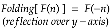
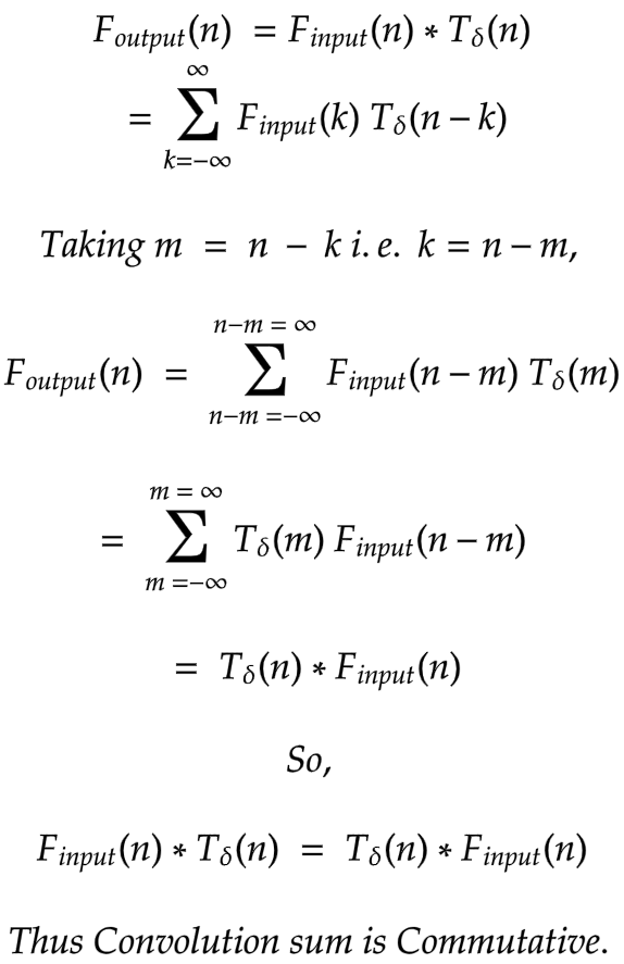
Commutativity of Convolution sum
|
|
In other words, if we excite a linear time invariant discrete-time system -
which has unit impulse response as Tδ - with Finput signal,
we get same response that we will receive when we excite another system -
which has unit impulse response as Finput - with Tδ signal.
|
|
|
»
|
|
Associativity of Convolution sum
|

|
|
|
|
»
|
|
Cascade connection and Convolution sum
|

|
|
|
|
»
|
|
Distributive law of Convolution sum
|

|
|
|
|
»
|
|
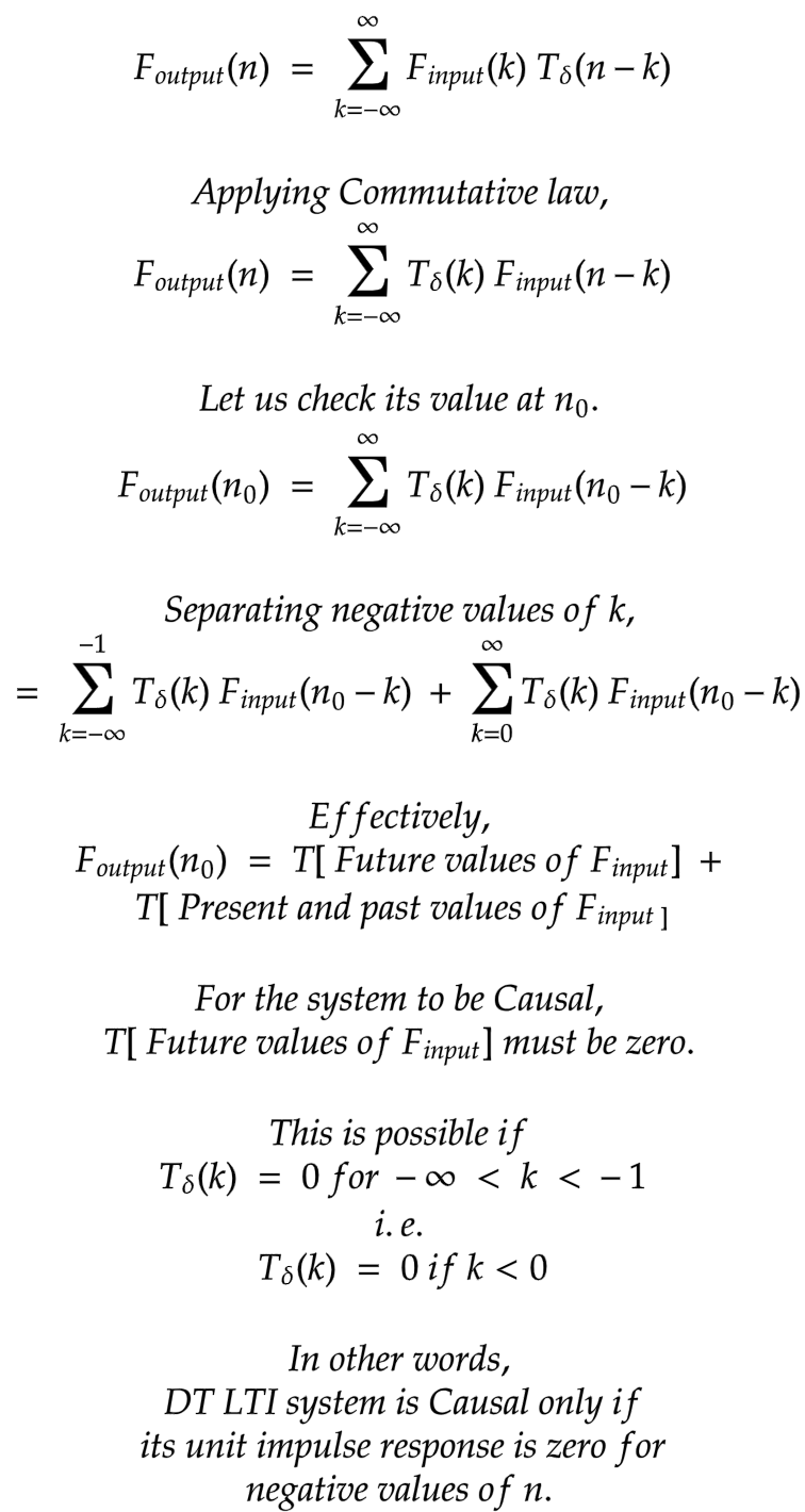
Check if system is Causal
|
|
|
|
|
»
|
|
Convolution sum for Causal systems
|

|
|
|
|
»
|
|
Check if system is Stable
|

|
|
|
|
»
|
|
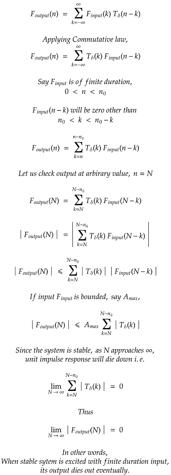
Response of stable system to finite duration input signal
|
|
|
|
|
»
|
|
Duration of unit impulse response
|

|
|
|
|
»
|
|
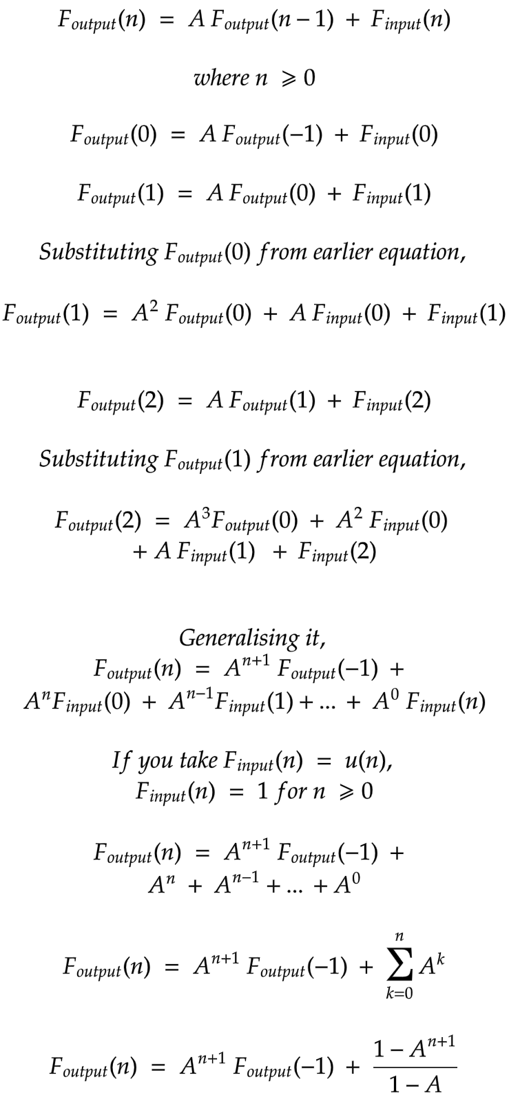
Recursive system
|

|
|
|
|
»
|
|
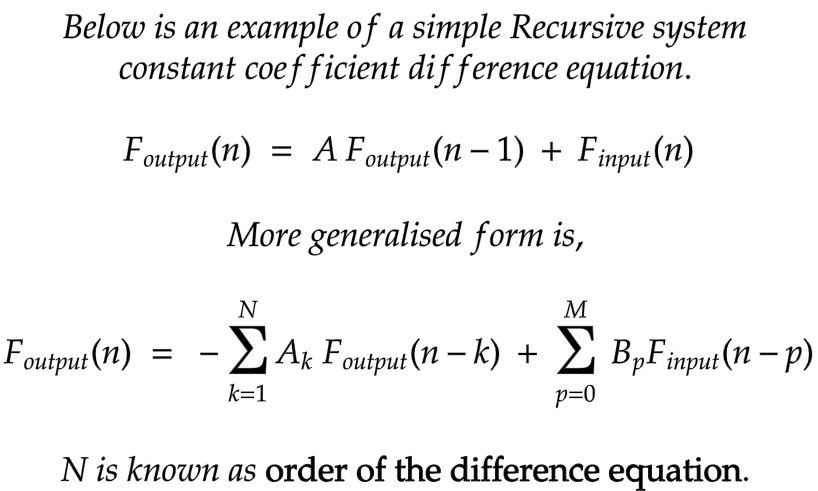
Constant coefficient difference equation
|
|
First term indicates that the system has a "State".
If the input is zero, first term is revealed.
So, it is known as Zero-Input Response (or Natural response).
Let us call it FZI.
It is obvious that if zero-input response is non-zero,
system has non-zero initial condition and
it is *not* relaxed.
Second term is revealed when FZI = 0 i.e.
when the system has no state or zero state.
So, the second term is known as Zero-State Response.
Let us call it FZS.
So,
|

|

|
It can be shown be that
recursive system decribed by a linear constant-coefficient difference equation is linear and time invariant.
|
|
|
»
|
|
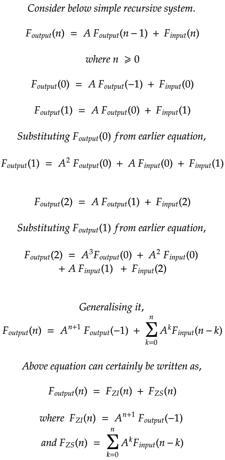
Example of a simple recursive system
|
|
Above equation indicates that FZS is convolution sum of Finput(n) and Anu(n)
(refer Convolution sum for Causal systems).
If the system is relaxed (i.e. FZI(n) = 0), FZS is same as the response of the system.
Combining above two points, we can say that the impulse reponse of above first-order recursive and relaxed system is Anu(n).
Another important point is: originally recursive, the system has been converted to non-recursive system !
The reverse should then be possible too.
In general, every FIR LTI system can be realised both recursively and non-recursively.
Let us check the stability of the system.
|

|
|
|
|
»
|
|
Solution of difference equation (direct method)
|
To find a solution to linear constant coefficient difference equation is
to find an explicit equation for Foutput in terms of its initial conditions for a particular input.
Below is a direct method.
|

|
Find homegeneous or complementary solution.
|

|
Example of finding homegeneous or complementary solution.
|

|
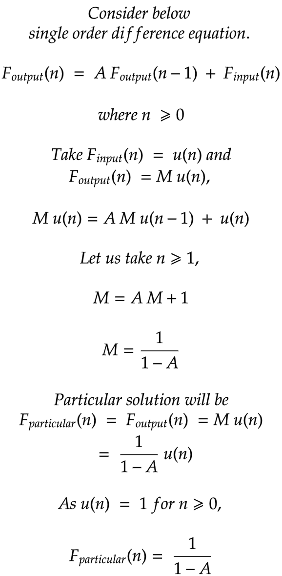
Now let us look at particular solution.
|

|
Example of finding particular solution.
|
|
Let us check full solution for our example.
|

|
Let us see if we get same solution by manual calculation.
|
|
Solutions from Manual calculation and that from Direct method match !
Another point to note here is that
the particular solution can be obtained from zero-state response by below equation.
|

|
Taking our example.
|

|
This matches with earlier calculated particular solution.
As particular solution is found by making n approach infinity,
it is called steady-state response.
The portion of the solution that dies out is called transient response.
|
|
|
»
|
|
Direct Form I and II realisations
|
|
Direct Form I is one way of realisation of LTI system described by linear constant coefficient difference equation.
The same can be converted to Form II.
|

|
|
Both forms will require same number of multiplcations (M + N + 1),
but Form II will require lesser number of delay elements.
Form I will require (M + N) delays whereas Form II will require max{M,N} delays.
|
|
|
»
|
|
Correlation of Discrete-Time Energy signals
|
As put in book Digital Signal Processing by Proakis and Manolakis,
"A mathematical operation that closely resembles Convolution is Correlation."
In Telecommunication, this concept could be applied to check whether (part of) the received signal match to reference signal (pattern) for 0 or 1.
Below equation describes Crosscorrelation between two discrete-time finite energy signals.
|

|
Let us check whether order of the signals matter in Crosscorrelation.
|

|
|
|
»
|
|
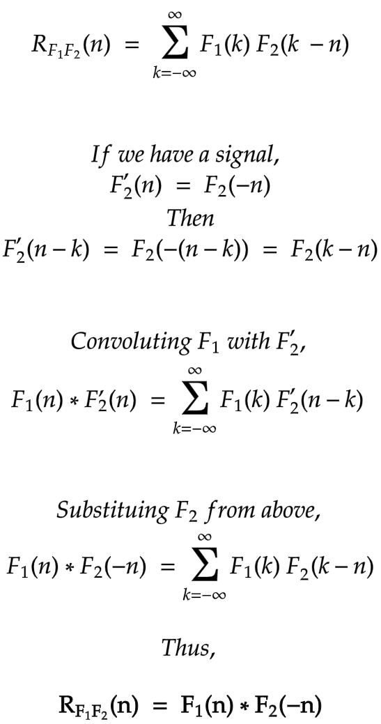
Crosscorrelation as a Convolution
|
Convolution and Crosscorrelation equations looks similar, here is how Crosscorrelation can be computed as a Convolution.
|
|
|
|
»
|
|
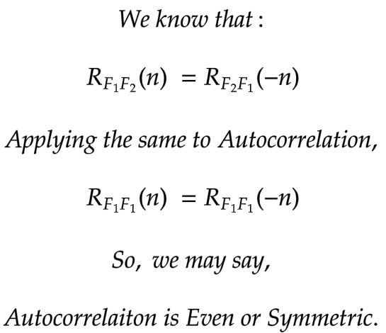
Autocorrelation
|
Autocorrelation is simply crosscorelation with itself, as shown below.
|

|
Here is another observation about Autocorrelation.
|
|
|
|
»
|
|
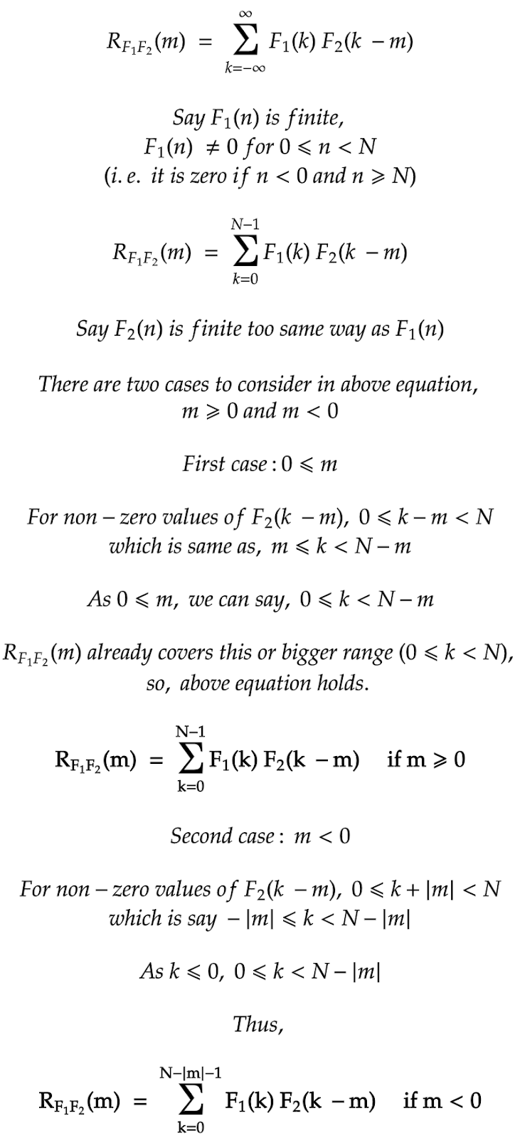
Crosscorrelation between finite duration discrete-time energy signals
|
In case of finite duration discrete-time energy signals, Crosscorrelation can be expressed as limited summation.
|
|
|
|
»
|
|
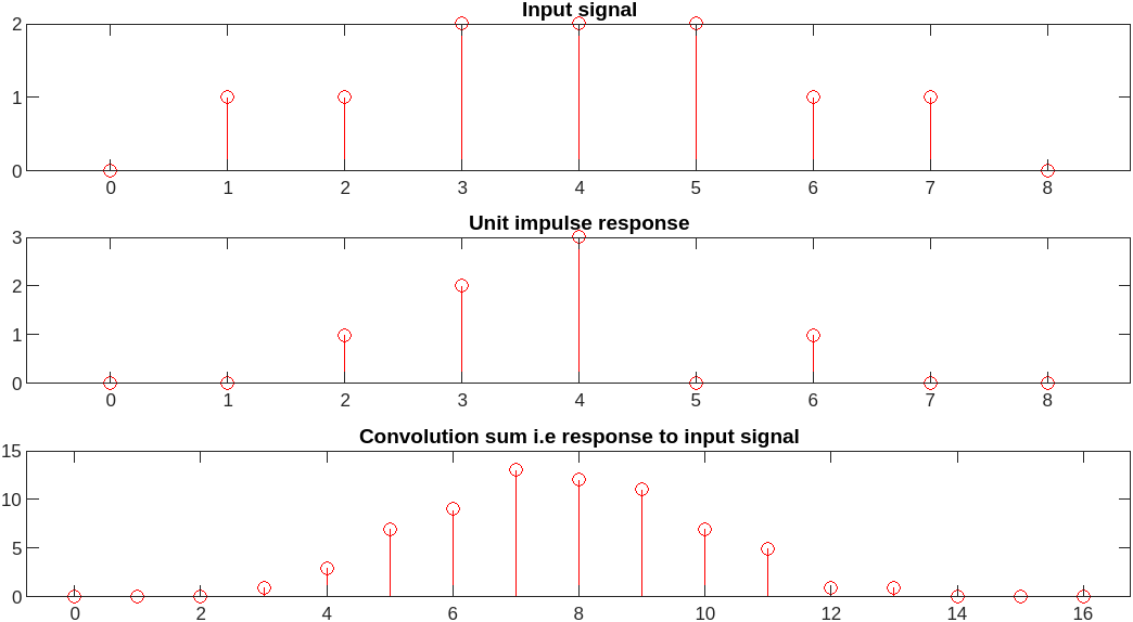
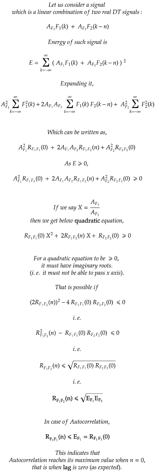
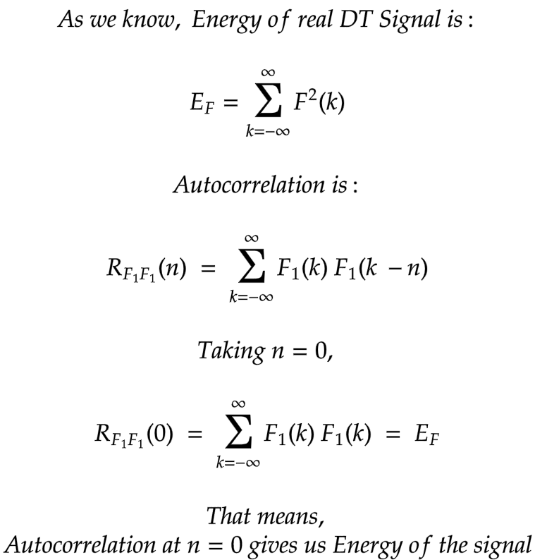
Autocorrelation and Energy of discrete-time energy signals
|
There is definite relation between Autocorrelation and Energy of discrete-time signals as shown below.
|
|
|
|
»
|
|
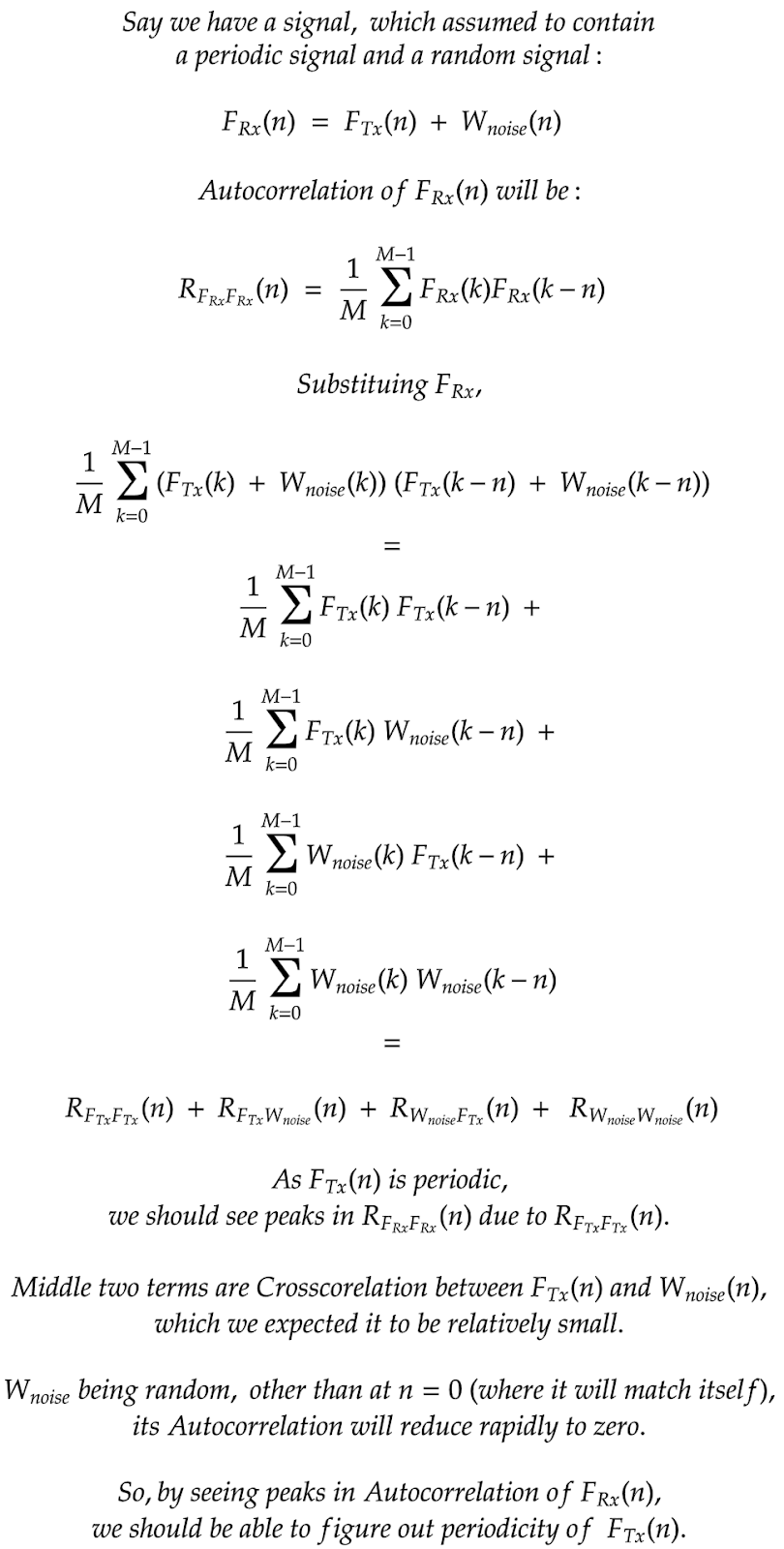
Correlation of discrete-time power signals
|

|
|
|
»
|
|
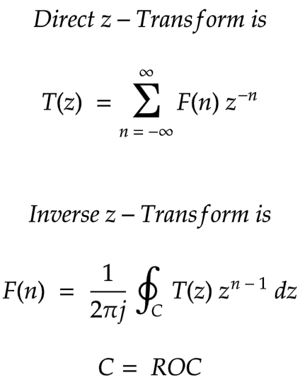
Direct z-Transform
|
|
"z" is a complex variable.
Above z-transform is also known as two sided or bilateral z-transform as it covers both negative and positive values of n.
For causal system, one sided and two sided would be identical.
ROC, Region of Convergence, is set of all values of z for which z-transform has finite values.
|
|
|
»
|
|
ROC
|

|
Above ROC analysis indeed holds true for common signals, considered above.
|
|
|
»
|
|
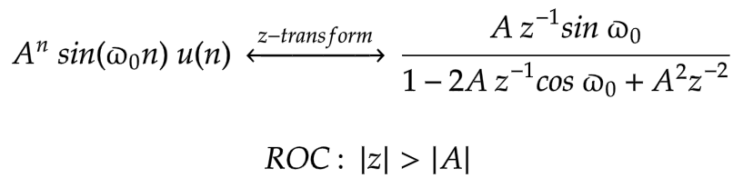
z-Transform of common signals collated
|

|
|

|
|

|
|

|
|

|
|

|
|

|
|

|
|

|
|
|
|
|
|
»
|
|
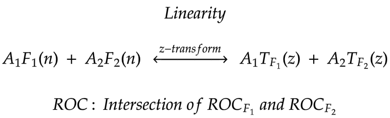
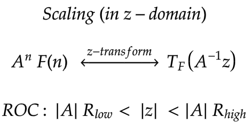
Properties of z-Transform
|

|
|
|
|

|
|
|
|

|
|

|
|

|
|

|
|

|
|

|
|

|
|

|
|

|
|
|
|
»
|
|
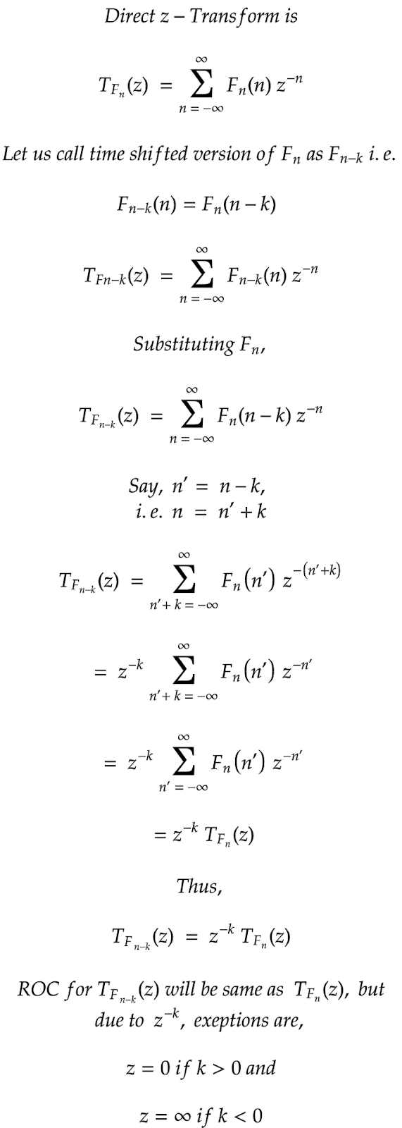
Proof for Time shifting property of z-Transform
|
|
|
|
»
|
|
Proof for Conjugation property of z-Transform
|

|
|
|
»
|
|
Collated observations and principals
|
Fundamental difference between continuous-time and discrete-time sinusoid signals is that
maximum rate of oscillation for discrete-time sinusoid signal is π !
In other words, discrete-time sinusoid signals with oscillation rate separated by 2π are identical.
More info here.
If we know frequency of input signal,
we can figure out another frequency
which will have identical sampled values for a given sampling frequency.
More info here.
Convolution sum implies that
if we know unit impulse response of the linear, relaxed, and time invariant discrete system,
we can calculate response of the system for arbitrary input signal by convolution sum of the input signal with unit impulse response of the system.
More info here.
If we excite a linear time invariant discrete-time system -
which has unit impulse response as Tδ - with Finput signal,
we get same response that we will receive when we excite another system -
which has unit impulse response as Finput - with Tδ signal.
More info here.
If two DT LTI systems interconnected in cascade fashion,
their combined unit impulse response is convolution sum of their individual unit impulse responses.
More info here.
If two DT LTI systems are connected in cascade fashion,
their order can be interchanged.
More info here.
If two DT LTI systems are connected in parallel fashion,
their combined unit impulse response sum of their individual unit impulse responses.
More info here.
DT LTI system is causal only if its unit impulse response is zero for negative values of n.
More info here.
DT LTI system is stable only if sum of its unit impulse responses is bounded.
More info here.
When stable system is excited with finite duration input, its output dies out eventually.
More info here.
FIR systems are said to have finite memory whereas IIR systems are said to have infinite memory.
More info here.
Recursive system decribed by a linear constant-coefficient difference equation is linear and time invariant.
More info here.
For a linear and time invariant recursive system to be stable, only a fraction of output must be taken in feedback.
More info here.
Every FIR LTI system can be realised both recursively and non-recursively.
More info here.
Direct Form II realisation requires lesser number of delay elements than Direct Form I realisation.
More info here.
As put in book Digital Signal Processing by Proakis and Manolakis,
"A mathematical operation that closely resembles Convolution is Correlation."
More info here.
Autocorrelation of Energy signal reaches its maximum value at n=0 and it is nothing but the energy of the signal.
More info here and here.
Correlation (both Crosscorrelation and Autocorrelation) are related to energy of Energy signal (and so power of the periodic signal).
More info here.
By Autocorrelation, we can find the periodicity of the periodic (power) signal mixed with random signal (say white noise).
More info here.
A discrete-time signal is uniquely determined by its z-transform and ROC of its z-transform.
More info here.
|
|
© Copyright Samir Amberkar 2018-24
| |
| |
|
|